Introduction
- Is the height of male (Age group 20-39 years old) in North America greater than 5.5 ?
- Is the average height of male (Age group 20-39 years old) in North America greater than 5.5 ?
- What is the average height of male (Age group 20-39 years old) in North America, Europe, and Asia ?
- Is the average height of male (Age group 20-39 years old) in North America different than in Europe or Asia ?
We often see similarly formatted questions statistics and use the concepts of inference and hypothesis testing to solve them. Inference and Hypothesis testing are the two most important and the most confusing concepts in statistics. Inference is related to estimating the population parameters from a sample. Hypothesis testing as its name suggests is a two step process, first is to build a hypothesis and second is to test how well our data support that hypothesis. Inference and hypothesis testing are highly interdependent on each other because the need to build a hypothesis before testing rises because we had to use inference in the first place. Therefore, the best way to understand them is by learning them together but understanding the fine differences between each other at the same time. We will decipher this mystery by solving to questions listed above by two different approach. First approach is a hypothetical situation where we will not use any inference and study the whole population while in the second approach we will do orthodox sampling and hypothesis testing.
Without using inference
Population is a data set representing all the entity of interest. For example: If we are interested in study of distribution of facebook users by country then, all 2.912 billion facebook users (facebook data 2022) constitute the population. At the same time if we are interested in distribution of facebook users in USA by state, then the facebook users in USA (307.34 million) constitute the population. Similarly, if we are interested in effect of age on hypertension in human being, then every single human being in world (7.9 billion, 2022) constitute our population. In situations where we are interested in small population like comparing the performance of two high school senior students only, we can make measurement on all students and compare the mean performance score in each school but such study will have very narrow scope and that result cannot be generalized to any other schools. Measurements made on a population are called parameters and mean is denoted by \(\mu\) and variance is denoted as \(\sigma^2\).
Now lets dive into our questions. If we are not going to use inference then we do not have our favorite option of sampling, we are forced to study the whole population. After some google search I could figure out that there are 450, 105 and 75 million males of this age group in Asia, Europe and North America respectively and each of these constitute a population for this question. Therefore, we will first need to find the height of each of these millions of people from each continent. We can simulate such population in R by generating a dummy population of such size and also calculate the mean, standard deviation and distribution for each population (Figure 1). Even for R, processing such large sized vector took quite a while, imagine you had to do this in reality. How much resource, money, time, and bookkeeping you would need to accomplish this?
set.seed(578)
Asia <- rnorm(4.5e8, mean=5, 0.2)
NorA <- rnorm(7.5e+07, mean=6.2, 0.4)
Euro <- rnorm(1.05e+08, mean= 5.7, 0.3)
mean_Asia <- mean(Asia)
var_Asia <- var(Asia)
hist_asia <-hist(Asia, breaks = 200, plot=FALSE)

mean_NorA <- mean(NorA)
var_NorA <- var(NorA)
hist_NorA <- hist(NorA, breaks= 200, plot=FALSE)

mean_Euro <- mean(Euro)
var_Euro <- var(Euro)
hist_Euro <- hist(Euro, breaks= 200, plot=FALSE)


plot(hist_asia, border="blue", col=NULL, xlim = c(4.2,7.5), xlab = "Continent",
     main="Distribution of height of male aged 20-39 in 3 different continents")
plot(hist_NorA, border = "red", col=NULL, add=TRUE)
plot(hist_Euro, border= "darkgreen", col=NULL, add=TRUE)
legend(5.5,8e6,
       legend = c(paste0("Asia (mean = ",round(mean_Asia,1), ", sd= ",round(sqrt(var_Asia),3),")" ),
                           paste0("Europe (mean = ",round(mean_Euro,1), ", sd= ",round(sqrt(var_Euro),1),")" ),
                           paste0("North America (mean = ",round(mean_NorA,1), ", sd= ",round(sqrt(var_NorA),1),")" )),
       fill= c("blue", "darkgreen", "red"))

For now lets assume, R did all that hard work for us and we have necessary data we wanted to collect and we can focus on the answers to the question above:
- Is the height of male (Age group 20-39 years old) in North America greater than 5.5 ?
We can see from figure 1 that most of the heights in North America is greater than 5.5. It may be tempting to answer “Yes” to this question but if we do so, we will be wrong because all the heights in North America are not above 5.5 (there is small proportion of heights in N America below 5.5). The alternative is to first calculate the probability of finding a height less than 5.5 (\(\alpha\)) in N America and re-phrase our answer as “the height in N America is greater than 5.5 but the probability that this is incorrect is \(\alpha\). The smaller this \(\alpha\) aka significance level or p-value gets there is more certainty in our answer. The generally acceptable value of \(\alpha\) is < 0.05. Since, we already know mean and sd of all these three population we can plug these number in pdf of normal distribution in R to find these p-values and also visualize the probability we are calculating as the area under the curve (figure 2). For details about probability distribution and how to calculate probabilities for normally distributed random variable see my notes on normal distribution and binomial distribution).
cat("Probability that heights in N. America is less that 5.5 is = ",
pnorm(5.5, mean= mean_NorA, sd= sqrt(var_NorA)), "\n")
cat("Probability that heights in Europe is less that 5.5 is = ",
pnorm(5.5, mean= mean_Euro, sd= sqrt(var_Euro)), "\n")
cat("Probability that heights in Asia is less that 5.5 is = ",
pnorm(5.5, mean= mean_Asia, sd= sqrt(var_Asia)), "\n")
curve(dnorm(x, mean=5, sd=0.2), from = 4,to= 7.5, col= "blue", ylab= "density", xlab="height(in)")
polygon(c(seq(4, 5.5, 0.05),5.5), c(dnorm(seq(4, 5.5, 0.05), mean =5, sd=0.2),0), col="lightblue")
curve(dnorm(x, mean=5.7, sd=0.3), col= "darkgreen",add=T)
polygon(c(seq(4, 5.5, 0.05),5.5), c(dnorm(seq(4, 5.5, 0.05), mean =5.7, sd=0.3),0), col="lightgreen")
curve(dnorm(x, mean=6.2, sd=0.4), col= "red", add=T)
polygon(c(seq(4, 5.5, 0.05),5.5), c(dnorm(seq(4, 5.5, 0.05), mean =6.2, sd=0.4),0), col="red")
curve(dnorm(x, mean=5, sd=0.2), col="blue", add = T)
legend(5.6,2,
       legend = c(paste0("Asia (mean = ",round(mean_Asia,1), ", sd= ",round(sqrt(var_Asia),3),")" ),
                           paste0("Europe (mean = ",round(mean_Euro,1), ", sd= ",round(sqrt(var_Euro),1),")" ),
                           paste0("North America (mean = ",round(mean_NorA,1), ", sd= ",round(sqrt(var_NorA),1),")" )),
       fill= c("blue", "darkgreen", "red"))
## Probability that heights in N. America is less that 5.5 is =  0.04006165

## Probability that heights in Europe is less that 5.5 is =  0.2524402

## Probability that heights in Asia is less that 5.5 is =  0.9937895

Using the p-values we can now give the complete answer; Yes, the height of male (Age group 20-39 years old) in N America is greater than 5.5 ft, given that this may be wrong 4% of the time. This 4% is below the generally accepted level of 5% error rate. Therefore, if a jeans manufacturer in N. America makes pants for height only above 5.5 ft, majority of man in N. America can find pants of their size. While a similar company in Europe would never want to manufacture pants that fit only above 5.5 ft because one fourth of its customers won’t be able to use that. Similarly, such company in Asia will manufacture pants that will fit heights less than 5.5 ft only. Therefore, although the answer we get using statistics may sound like incomplete information it has a lot of practical application when the result needs to be implemented in a large population.
Lets review what we did here because it forms the foundation of any hypothesis testing. When the underlying distribution of a random variable (Y) is known, for any value of that random variable (y), we can find the probability of observing values more extreme than that value(y). If that probability is very small, then we can say, that value(y) itself is very rear in this distribution and could belong to other distribution. To take an example from the problem we are working with, we saw that probability getting a height greater than 5.5 in Asia is extremely low (0.00063). Therefore, if we randomly sample a man from the whole world and his height is found to be 5.5, then we can very confidently (probability of error is only 0.00063) say he is not from Asia. Does this mean he belong to N America? Or Europe? No, we will never know that answer but the point is when we properly select the random variable(Y) (sample mean, difference of sample mean, sample variance, sample proportion etc. ) and ask the correct question we can get some very useful answers about question of interest. Once we understand this we will later see how aptly early statisticians have devised hypothesis testing to get best out of it.
- Is the average height of male (Age group 20-39 years old) in North America greater than 5.5 ?
Since we have made measurements on every man in that age group we can find the true mean by calculating sum of all the heights in a continent and divide by the population size of that continent which R already did for us. The mean height in N America is 6.2. This is true mean of this population so we do not need to make any estimate or confidence intervals to say that mean height in N America is greater that 5.5.
- What is the average height of male (Age group 20-39 years old) in North America, Europe, and Asia ?
Similar to question no. 2, since we have complete population data, we can say with 100% confidence that mean height in N America, Europe and Asia is 6.2, 5.7 and 5 respectively.
- Is the average height of male (Age group 20-39 years old) in North America different than in Europe or Asia ?
Answer to this is also straight forward. From question no 3 we can see clearly, they are different for these three populations.
We saw, many of these questions could be easily answered because we could measure each and every man and get true mean \((\mu)\) and sd \((\sigma)\) for these populations. But recall again how arduous that task could be and the real-world situation is even more complicated by the fact that most populations we need to study have infinite numbers of entities, so it is impossible to find the true population parameters.
This is where inference shines in. Inference provides the unbiased estimate of the population parameters using the information from a sample of certain size (n) from that population. Now, that we know the complications of studying the whole population we will see below, how we can deal with our question in much practical way using principles of inference and hypothesis testing, but first lets understand how inference works in general.
Statistical inference
sample is a subset of population (size = n) and is unbiased representation of the population. If n= \(\infty\), sample behaves like the population and if n = 1, sample is just one observation from the population. It is very important for sample to be a representative of population because ultimately measurements made on a sample will be used to infer the population parameter. Any measurements made on a sample is called statistic (note statistics is branch of mathematics which study these statistic). For example sample mean (\(\bar x\)) and sample variance (\(s^2\)) are two most important sample statistic.
Sample is the main workhorse of statistics. This is all we have to make inference about population parameters. Usually a sample used to make inference on population parameters is much smaller in size than the population itself so it is very convenient to collect data (statistic) on a sample but this convenience comes at some cost, which is uncertainty associated with the estimate. We will see later, this uncertainty depend on population variance and we can tackle it by increasing sample size (n). Fortunately, in many real life situation, a sample of small size gives an estimate of population parameters with high precision. Therefore in a statistical analysis, sample statistic is used to make a statement about the population parameter which is always accompanied by a degree of precision (or chances of making an error). In situations where, the precision is relatively high (chances of making an error is low) we trust that statement and interpret our experiment based off that statement about population. On the other hand, if precision is low (chances of making an error is high), we do not trust that statement about population, so we cannot make any interpretation about the experiment or question of interest. The widely accepted level of that accuracy in scientific community is above 95% (or less than 5% chances of making an error).
Inference framework
Statistical inference uses very complex mathematical models to build a framework which will take the information from a sample of finite size (n) as an input and output estimate of parameters for the population of infinite size (along with degree of uncertainty). Then we can use these estimates of population parameters for the purpose of hypothesis testing or other interpretation downstream. Although, we are not interested in details of the mathematical models we must see what are the major components of this framework and how it process the information from a sample and what assumptions must be satisfied for the results from this framework to be valid.
#population defined by mean and variance
poplist <- list(pop1=c(5, 0.04) , pop2= c(5.7, 0.0898), pop3 = c(6.2, 0.1599))
pop_col = c("blue", "darkgreen", "red")

plot(x=0,y=0,xlim= c(4,7.5), ylim=c(0,2), pch=NULL,  ylab= "density", main="Distribution of 3 populations", yaxt="n")
for(i in seq_along(poplist)){
  curve(dnorm(x, mean=poplist[[i]][1], sd=sqrt(poplist[[i]][2])), col=pop_col[i], lwd=2,add=T)
}
#Standardized normal curve
curve(dnorm(x), from = -4,to= +4, ylab= "density", xlab= "z", main= "Standard normal distribution", yaxt="n", lwd=1.7)
##Sampling distribution of sample mean
sample_size <- c(5, 15, 25, 50)
sample_colors <- list(pop1= c("#89CFF0","#6495ED","#6082B6","#5D3FD3"),
                      pop2= c("#AFE1AF","#50C878","#008000","#355E3B"),
                      pop3= c("#F88379","#C04000","#E30B5C","#A52A2A"))
plot(x=0,y=0,xlim= c(4,7.5), ylim=c(0,13), pch=NULL,xlab="sample mean",  ylab= "density", main="Sampling distribution of sample mean", yaxt="n")
for(i in seq_along(poplist)){
  for(sample in seq_along(sample_size)){
  curve(dnorm(x, mean=poplist[[i]][1], sd=sqrt(poplist[[i]][2]/sample_size[sample])), col=sample_colors[[i]][sample],lwd=1.7, add=T)
}
}
###sampling distribution of sample variance
# When sample size is close to 30 or more chi square distribution is similar to normal distribution
plot(x=0,y=0,xlim= c(0,0.4), ylim=c(0,24), pch=NULL,xlab="sample variance",  ylab= "density", main="Sampling distribution of sample varaince ", yaxt="n")
for(i in seq_along(poplist)){
  for(sample in 3:4){
  curve(dnorm(x, mean=poplist[[i]][2], sd=sqrt((poplist[[i]][2])^2/(sample_size[sample]-1)*2)), col=sample_colors[[i]][sample],lwd=1.7, add=T)
}
}
####Plot chisquare for distribution
plot(x=0,y=0,xlim= c(0,65), ylim=c(0,0.2), pch=NULL,xlab="Chi square",  ylab= "density", main="Chi-square distribution ", yaxt="n")
linecol <- rainbow(4)
size = c(5,15,25,50)
for(i in 1:length(size)){
    curve(dchisq(x, df=size[i]-1), from = 0,to= 65, col= linecol[i], add = T, lwd=1.7)
}
legend(30,0.2, legend = c( paste0("df = ", size-1 )), col= c(linecol), lty= c(1,1,1,1))
###Plot t-distribution
plot(x=0,y=0,xlim= c(-4,4), ylim=c(0,0.4), pch=NULL,xlab="t-statistic",  ylab= "density", main="t-distribution ", yaxt="n")
linecol <- rainbow(4)
size = c(5,15,25,50)
for(i in 1:length(size)){
  curve(dnorm(x), from = -4,to= 4, col= "darkgreen", ylab= "density", add=T, lwd=1.7)
    curve(dt(x, df=size[i]-1), from = -4,to= 4, col= linecol[i], add = T, lwd=1.7)
}
legend(2,0.4, legend = c("Std. Normal", paste0("df = ", size-1 )), col= c("darkgreen",linecol), lty= c(1,1,1,1,1))
##### F-distribution
plot(x=0,y=0,xlim= c(0,3), ylim=c(0,1.5), pch=NULL,xlab="F-statistic",  ylab= "density", main="F-distribution ", yaxt="n")
linecol <- rainbow(4)
size1 = c(5,15,25,50)
size2 = c(10,23,4,50)
for(i in 1:length(size)){
    curve(df(x, df1=size1[i]-1, df2=size2[i]-1), col= linecol[i], add = T, lwd=1.7)
}
legend(2,1, legend = c( paste0("df1 = ", size1-1, ", df2 = ", size2-1  )), col= c(linecol), lty= c(1,1,1,1))
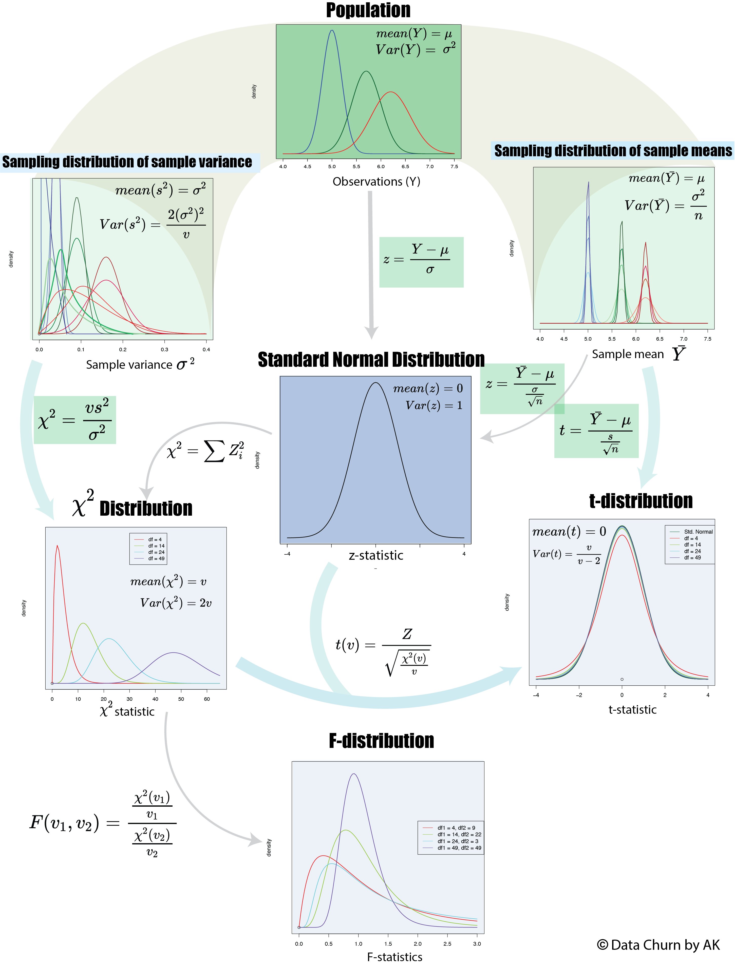
We need to acknowledge that population parameters (\(\mu\)) and (\(\sigma^2\)) are fixed and universal quantity and we will never know its true value (We will use the population parameters from our simulated data to illustrate the concepts only). The ultimate goal of inference is to get best estimate of these two parameters using only statistic calculated from a sample of size = n. The major components of the statistical framework are shown in figure 3. The population with mean (\(\mu\)) and variance (\(\sigma^2\)) is on the top of this framework and it is represented by distribution of random variable we are interested in (Example height of male aged between 20-39). The most important assumption about the population is that it follows normal distribution hence a standard normal distribution curve can be used to find probabilities related to the population.
Two most important statistic we measure on a sample is sample mean \((\bar x)\) and sample variance \((s^2)\). Central Limit Theorem gives the distribution of sampling distribution of sample mean which states that sample mean are also normally distributed and mean of such distribution is also population mean (\(\mu\)), but has less variance than the population variance (figure 3) given by \(\frac{\sigma^2}{n}\). Therefore, larger the sample size gets less is the variance (shown by darker color for each population in figure 3). To get the probability associated with this distribution we can do a z-scale transformation for which we need population mean \(\mu\) and population variance \(\sigma^2\).
\[z= \frac{\bar Y- \mu}{\frac{\sigma}{\sqrt n}}\]Hypothesis testing is designed in such a way that our question will have the population mean (some number we are comparing sample mean to, or 0 when we are comparing two populations) but we should be able to estimate the population variance using the sample variance. The top left plot in figure 3 show the distribution of sample variance. It is found that sample variance follows Chi-squared \(\chi ^2\) distribution. Which shows, mean of the distribution of sample variance is population variance but unlike sample mean, when the sample size is small it is heavily skewed on the left and the shape of distribution depends on the degree of freedom. Which means sample variance calculated from a random sample of small size most probably gives the underestimate of the population variance. \(\chi ^2\) distribution accounts for this discrepancy by providing separate distribution for samples of different size. To include this information in our z-score calculation a new statistic is calculated called t-statistic which follows t-distribution and similar to \(\chi^2\) distribution it has different distribution for different sample size. Both \(\chi^2\) and t-distribution have same shape as normal distribution when the sample size is greater than 30. Once we have this t-statistic we can use the probability given by t-distribution to find any probability associated with sampling distribution of sample means.
\[t-statistic = \frac{\bar Y- \mu}{\frac{s}{\sqrt n}}\]As you can see the all the variables in the equation can be calculated using a sample which enables us to compare the sample mean with the mean given in the question, when we consider a hypothetical population with \(\mu\) = mean given by question and the sample we are working with is a sample from that population.
The above method works best only when we need to compare two means. When we need to compare means from more than one population ANOVA is used for which inference framework has F-distribution which is basically ratio of two variance. If the variance is equal it has a value of 1 other wise it will be greater than 1. Details in ANOVA.
Application
Now that we have seen the basic components of inference, we can revisit our questions we are working on. ( NB: Please see notes focused on each distribution to learn more about them)
- Is the height of male (Age group 20-39 years old) in North America greater than 5.5 ?
We could answer this question in much detail when we had the distribution of heights (defined by population mean and variance) in hand. But now we do not know population parameters hence inference is not able to provide answer to this question. This is one of the limitations of inferential statistics, rather than each observation we will be only focusing on the mean of populations, so we can still answer other questions below.
- Is the average height of male (Age group 20-39 years old) in North America greater than 5.5 ?
Lets recall what we learned about hypothesis testing in the beginning. If we know the underlying distribution of a random variable we can check, how unusual a given value is to that distribution and if it is indeed very rare to observe that value in given distribution we can conclude, that value does not belong to the given distribution. In hypothesis testing we do exactly same but in little twisted way to be able to use the inference framework discussed above. In this setup we make a null hypothesis and it is exactly opposite to what we want in our question of interest. So why we need this null hypothesis? To answer this, lets see what is our question and what information we have about our population. Since we are not measuring every man living in N America, all we can do is measure heights in a randomly selected sample of size(n). Then, the mean we calculate from this sample(\(\bar x\)) is just one value in the sampling distribution of the sample means for this population. We cannot calculate t-statistic with just sample mean and sample variance. We need the population mean. The question is giving us some clue. What you should visualize in your mind is that there are two populations in this question. The height of male (Age group 20-39 years old) in N America is the first and obvious population we have been seeing from the beginning, but the number we are tying to compare (5.5) is actually mean of a hypothetical population. Therefore, if we cannot calculate the population mean for our population, we can assume that our sample is taken from that hypothetical population (for which mean is given by the question) and check how unusual is this sample mean in that hypothetical population? If it comes out to be a rare event than we can reach to the conclusion that our sample does not belong to that hypothetical population.
What we are doing by assuming our sample came from that hypothetical population given by question is building a null hypothesis. And at the end of the test we want to see the sample mean we get from our sample, to be a rare event for that hypothetical population. Which means we reject null hypothesis.
To formally do this we first state the null hypothesis (\(H_o\)) and alternate hypothesis (\(H_1\))
\[H_o: \mu = 5.5\] \[H_1: \mu >5.5\]Then calculate the t-statistic
\[t =\frac{\bar x - 5.5}{\frac{s}{\sqrt n}}\]##Lets first make a sample of 100 from the population of NoA
set.seed(45)
set1 <- sample(NorA, 100)
cat("The t-statistic for this test is = ",(mean(set1)-5.5)/sqrt(var(set1)/100), "\n")
cat( "The p-value for this test is = ",pt((mean(set1)-5.5)/sqrt(var(set1)/100), 99, lower.tail = FALSE), "\n \n")
cat("##########--USING R t.test FUNCTION --########\n")
t.test(set1, mu= 5.5, alternative = "greater")
## The t-statistic for this test is =  18.31421
## The p-value for this test is =  7.324508e-34
##
##
## ##########--USING R t.test FUNCTION --########
##  One Sample t-test
##
## data:  set1
## t = 18.314, df = 99, p-value < 2.2e-16
## alternative hypothesis: true mean is greater than 5.5
## 95 percent confidence interval:
##  6.147978      Inf
## sample estimates:
## mean of x
##  6.212581
##visualize
##BIG ASSUMPTION JUST FOR VISUALIZATION
#for hypothetical population the variance is assumed to be equal to sample variance (just an approximation to see big picture )
plot(x=0,y=0,xlim= c(3,9), ylim=c(0,11), pch=NULL,  ylab= "density", main="Distribution null hypothesis and alternative", yaxt="n")
curve(dnorm(x, mean=6.2, sd= sqrt(var_NorA)), col="#f4c2c2", lwd=2,add=T)
curve(dnorm(x, mean=6.2, sd= sqrt(var_NorA/100)),n=500, col="red", lwd=2,add=T)
curve(dnorm(x, mean=5.5, sd= sqrt(var(set1))), col="#d2d1f9", lwd=2,add=T)
curve(dnorm(x, mean=5.5, sd= sqrt(var(set1)/100)), n=500,col="purple", lwd=2,add=T)

abline(v=5.5, col="#d2d1f9" )
abline(v=6.2, col="#f4c2c2", lwd=2 )
abline(v= mean(set1))

In the figure 4 we can clearly see, why p-value is so small. The distribution with green shade and the green dot at 6.21 are the only one distribution and data that is given to us by the question. The alternative hypothesis and other populations are shown using the data we collected from first section just to show big picture.
- What is the average height of male (Age group 20-39 years old) in North America, Europe, and Asia ?
In absence of the knowledge of true population mean, the mean we get from a sample is the best estimate of the true population mean. But given the inherent variability in the sampling distribution of sample means there will be some level of uncertainty. To account for this instead of reporting the point estimate, we find a interval at certain significance level based of the sample mean. Lets start with North America, we will again randomly take a sample of size(n)= 50. And calculate the sample mean of this sample. Since we do not know the population mean, we will need to assume the population mean is sample mean in this sample and based off the distribution centered around this sample mean we will calculate the range of sample means which is encompass 95% of the sample means(exclude only 2.5% means on both extremes of distribution). Narrower this interval is better is the quality. The interpretation for CI at 95% significance, is 95% of the times we construct such intervals, true means will be within that interval.
set.seed(100)
set2 <- sample(NorA, 50)
mean_set2 <- mean(set2)
mean_set2 - (qt(0.025, 49, lower.tail = FALSE)*sqrt(var(set2)/50))
mean_set2 + (qt(0.025, 49, lower.tail = FALSE)*sqrt(var(set2)/50))
#Results can be confirmed by doing a test test for this mean
t.test(set2, mu= mean_set2, alternative = "two.sided")
## Lower limit is  6.169956
## Higher limit is  6.405479
## ####---Using the function available in R ------#####
##  One Sample t-test
##
## data:  set2
## t = 0, df = 49, p-value = 1
## alternative hypothesis: true mean is not equal to 6.287718
## 95 percent confidence interval:
##  6.169956 6.405479
## sample estimates:
## mean of x
##  6.287718
##visualize
##BIG ASSUMPTION JUST FOR VISUALIZATION
#for unknow population with mean equal to sample mean  the variance is assumed to be equal to sample variance (just an approximation to see big picture )

plot(x=0,y=0,xlim= c(5,7.3), ylim=c(0,11), pch=NULL,  ylab= "density", main="Distribution null hypothesis and alternative", yaxt="n")
polygon(c(seq(6, 6.5, 0.005),0), c(dnorm(seq(6, 6.5, 0.005), mean =mean_set2, sd=sqrt(var(set2)/100)),0), col="lightblue")
curve(dnorm(x, mean=6.2, sd= sqrt(var_NorA)), col="#f4c2c2", lwd=2,add=T)
curve(dnorm(x, mean=6.2, sd= sqrt(var_NorA/100)),n=500, col="red", lwd=2,add=T)
curve(dnorm(x, mean=mean_set2, sd= sqrt(var(set2))), col="#d2d1f9", lwd=2,add=T)
curve(dnorm(x, mean=mean_set2, sd= sqrt(var(set2)/100)), n=500,col="purple", lwd=2,add=T)

abline(v=mean_set2, col="#d2d1f9" )
abline(v=6.2, col="#f4c2c2", lwd=2 )
lines(c(6.1699, 6.4054), c(5,5))
 The figure above show the hypothetical population around the sample mean from our sample (shaded blue color) and its relation to true sampling distribution of mean (red). Also at the bottom somewhat flat is the distribution of height. The black line is the 95% confidence interval and even for this sample we can see the true population mean lies within this interval.
- Is the average height of male (Age group 20-39 years old) in North America different than in Europe or Asia ?
This is the question about comparing two populations of sample means. Therefore we need to polish our approach little bit. We now know that, for each populations we can build a sampling distribution of sample means, them mean of such distribution is the true mean of the population. When we need to compare two population we will have two such distributions of sampling means. As we have see so far, ultimately, we will need only one distribution and a value to see how uncommon it is in that distribution. Therefore, in case of comparing two populations we need to first find distribution for a random variable which is the difference between the sample means of two populations. The random variable \(\bar Y_1 - \bar Y_2\) also follows t-distribution and the t-statistic for large sample size is calculated by this formula:
\[t = \frac{\bar y1- \bar y_2}{\sqrt{\frac {s_1^2}{n1}+\frac{s_2^2}{n_2}}}\]set.seed(500)
## is there difference between N. America and Asia
cat("####----T-test between N America and Asia---------######\n")
Sample_NAmerica <- sample(NorA, 50)
Sample_Asia <- sample(Asia, 50)
t.test(Sample_Asia, Sample_NAmerica, )
## see for N. America and Europe
cat("####----T-test between N America and Europe---------######\n")
Sample_Euro <- sample(Euro, 50)
t.test(Sample_Euro, Sample_NAmerica)
## ####----T-test between N America and Asia---------######
##
##  Welch Two Sample t-test
##
## data:  Sample_Asia and Sample_NAmerica
## t = -17.984, df = 69.395, p-value < 2.2e-16
## alternative hypothesis: true difference in means is not equal to 0
## 95 percent confidence interval:
##  -1.306438 -1.045557
## sample estimates:
## mean of x mean of y
##  5.006745  6.182742

## ####----T-test between N America and Europe---------######
##
##  Welch Two Sample t-test
##
## data:  Sample_Euro and Sample_NAmerica
## t = -6.0688, df = 92.631, p-value = 2.792e-08
## alternative hypothesis: true difference in means is not equal to 0
## 95 percent confidence interval:
##  -0.6059330 -0.3071451
## sample estimates:
## mean of x mean of y
##  5.726203  6.182742
Conclusions:
Using the methods of inference we are able estimate the population parameters with much more accuracy even with very small amount of data. This note provides only the overview of different hypothesis testing possible in statistics but hope this provided a clear concept of big picture of what is going on when we do a hypothesis testing.