Expected value

Expected value of a random variable

Frequently called Expected value, expectation, expectancy, mathematical expectation, sometime referred simply as mean, average or first moment. For a random variable X it is found to be represented by any one of these symbols \(\text{ E(X), E[X], EX, E, \mathbb{E} }\).

Definition

Once we know the probability distribution of a random variable we can find the expected value of that random variable, which is exactly what the name is suggesting, it is average or mean value of the random variable which we expect to find most often. Lets plot binomial probability distribution of two random variables (X and Y) with same number of trials but different p.

par(mfrow=c(1,2))
random_var <- 0:10
probability <- NULL
for (i in 1:11) {
  k=random_var[i]
  #probability[i] <- choose(10, k)*(0.2^k)*(0.8)^(10-k)
  probability[i]<- dbinom(k, size=10, prob = 0.2)
}

barplot( probability, names.arg = random_var, main = 
           "B(X~10,0.2)", 
         xlab= "random variable, X", ylab= "probability")
#Next binomial probability 
random_var <- 0:10
probability <- NULL
for (i in 1:11) {
  k=random_var[i]
  #probability[i] <- choose(10, k)*(0.2^k)*(0.8)^(10-k)
  probability[i]<- dbinom(k, size=10, prob = 0.7)
}

barplot( probability, names.arg = random_var, main = 
           "B(Y~10,0.7)", 
         xlab= "random variable, Y", ylab= "probability")

done!

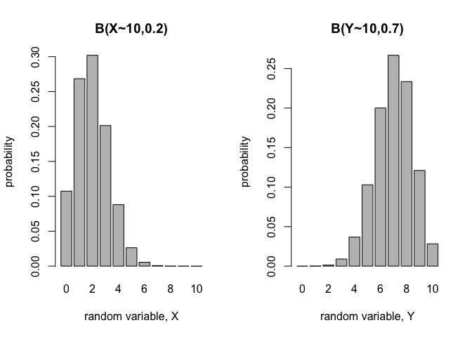So for the plot we can see that X, is most often expected be 2 and Y is most often expected to be 7. Therefore,

\[E[X] = 2\]

and

\[E[Y] = 7\]

Finite probability distribution

Now lets see how to it is calculated mathematically. For a random variable, X with finite probability distribution the expected value of X, E[X] is equal to the weighted mean of all possible outcomes (note that random variables are always numeric values). For example in binomial distribution \((X \sim B(n,p))\) we have only n+1 number of possible outcomes (k) each with probability of P(X=k) defined by following equation:

\[P(Y=k)= {n \choose k}p^k(1-p)^{n-k}\]

Therefore, when we calculate the weighted average of all outcomes \(k\), (weighted by their probability) then it is the expected value of random variable X.

\[E[X] = \sum_{k=0}^n k.{n \choose k}p^k(1-p)^{n-k}\]

On further solving the equation this simplifies to

\[= np\]

For continuous density function

Random variables like sample mean which follow normal distribution which is a continuous probability density function the expected value needs to be calculated by using integration but concept can be understood as similar to above discussed for binomial distribution.

Wikipedia has elaborate explanation about expected value of different probability distribution wiki Check the table half way in this page.